FX Quant > Numerical Simulations and Evidence of Profitability
Below are given return-leverage graphs for the Fx Quant 11 strategy (V.10/2008), which started live trading on November 1, 2008. Actual trading results after this date (until August 2011, when v.10/2008 was replaced by v.08/2011) can be found on the FXQ Real Performance page.
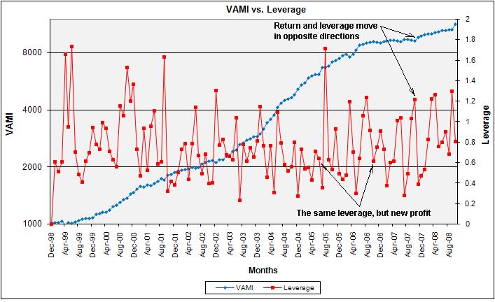
Figure 1. A very important feature of the Fx Quant 11 system is stationarity, or mean-reversion, of the system leverage. We define the system leverage as a ratio of the total long currency exposure (all long portfolio components, USD denominated) to Net Asset Value (NAV). Numerical experiments show that the leverage oscillates/ reverts to its long term average of 0.77. This can help us determine the optimal timing to start trading (or NOT to start trading). The system either: 1.) makes a new profit (the leverage decreases), or 2.) the leverage increases (the equity curve temporarily retraces).
As time passes, the leverage oscillates around its mean, BUT the return makes a new high - see the diagram above.

Figure 2. We define the crossover VAMI (the red line in diagram above) as a value of VAMI when the leverage crosses over the mean leverage of 0.77. Note that the crossover VAMI monotonically rises on every leverage crossover. Although the leverage goes up and down all the time, it eventually reverts and crosses over its mean (0.77), making a new VAMI high on each crossover. This is a strong evidence of profitability of the system; as long as the leverage reverts to mean (at least it did so in the past), the system makes new profit. The above graph shows that, however large the drawdown and leverage are, the system recovers from losses and sets a new VAMI peak. Sometimes it takes months (and large losses in account), but patience is needed to see a new profit.
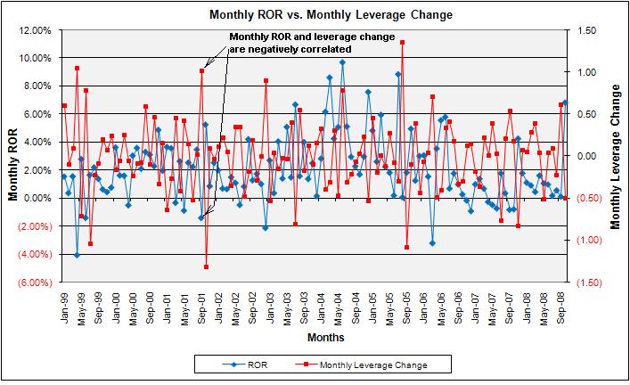
Figure 3. There is a very strong negative correlation between the monthly rate of return (ROR) and the month-to-month (MTM) leverage change. An increase in monthly leverage, however, produces not as sharp drop in monthly ROR. The opposite also holds true: a positive monthly ROR does not decrease the leverage as much as a negative ROR increases the leverage (see the graph below).
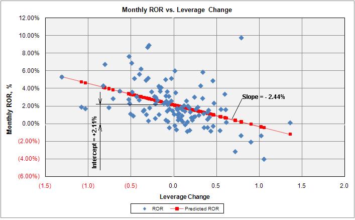
Figure 4. The correlation between the monthly ROR and leverage change can mathematically be described as:
Predicted Monthly ROR = 2.115% - 2.44% x Leverage Change
Let us sum the above formula across all months from the testing interval. Leverage changes will cancel each other, i.e. their sum will be zero (remember the leverage change has a zero mean) and we come to conclusion that
Cumulative ROR = Sum(Monthly RORs) = N x 2.115% = 118 x 2.115% = 249.6% (non-compounded)
where N=118 is the number of months in the testing interval
Hence the Average Predicted Monthly ROR = 2.115% (look at the intercept on the Monthly ROR axis). This correlation was persistent and the intercept was always positive, regardless the choice of system parameters. This brings us to a conclusion that, in long run, the system should be profitable, if a reasonably large leverage is used. Using too large a leverage can deplete the trading account, despite the long term system profitability.
You can open this Excel table and click on the Drawdown & Corel. Analysis and ROR vs. Lever. Change tabs to see calculations for the latest version of the system (V.10/2008) .
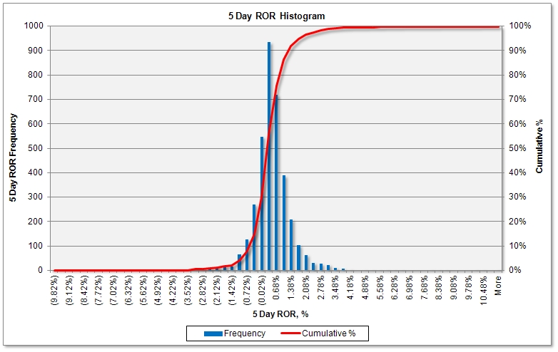
Figure 5. 5-Day ROR Histogram
The above histogram shows that:
1. There is very regular, bell-shaped, thin tailed distribution of 5-day rolling rates of return . Robust systems, which are not curve-fitted usually have this type of distribution.
2. The 5-day rolling rate of return (ROR) mean is positive and equals 0.37%. There is a 50% probability that the 5-day rate of return will be greater than 0.37% and 50% probability the return will be less than 0.37%.
3. 5-Day RORs are more clustered in the positive territory in the histogram above. There is a 28.5% probability that a 5-day ROR will be negative and a 71.5% probability the 5-day ROR will be positive.
4. The 5-day Value-at-Risk (VaR) for the 95% confidence level is 1.01%. This means that the risk of loss in a 5-day period is 1.01%, with a 95% probability. The probability of loss of more than 1.01% in a 5 day period is 5%. Similarly, the 5-day VaR for the 99% confidence level is 2.20%. Excessive negative RORs do and will happen, although with decreasing probability. To see these calculations open the 5 Day ROR Percentile tab in this Excel workbook.
Detailed actual and backtesting performance reports can be found in the FXQ Real Performance and FXQ Back testing section of our web site.